Estimate a-value#
The a-value is the parameter in the Gutenberg-Richter law that contains information on the rate of seismicity within the volume and time interval of interest.
Here, we
Explain the basics of a-value estimation, and
Show the different methods that a-value estimation can be done with SeismoStats.
1. Short Introduction on a-value Estimation#
The GR law above the completeness magnitude \(m_c\) can be expressed as
where \(N(m)\) is the number of events with magnitudes larger than or equal to \(m\) in a given catalog, and \(a\) and \(b\) are the a-value and b-value, respectively. With this definition we can estimate the a-value as the base 10 logarithm of the number of earthquakes above completeness:
There are, however, two commonly used modifications of the function above, which are relevant if we want to compare different a-values to each other.
1.1 Reference Magnitude#
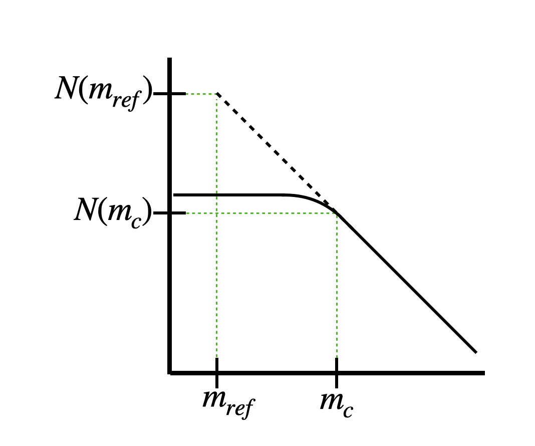
First, it might be that the level of completeness is not the same for different catalogs to be compared. Therefore, in practice, many estimate the a-value with respect to a certain reference magnitude, such that \(10^{a_{m_{ref}}} = N(m_{ref})\). Here, \(N(m_{ref})\) is not the actual number of earthquakes above \(m_{ref}\), but the extrapolated number if the GR law were perfectly valid above and below \(m_c\), as shown in Fig. 1. This reference a-value can be estimated using the a-value defined in Eq. (1): \(a_{m_{ref}} = a - b(m_{ref} - m_c)\).
1.2 Scaling#
Second, the time intervals of two catalogs that are compared are often not the same, making it hard to compare. To standardize the comparison, researchers often scale the a-value so that \(N(m)\) represents the number of earthquakes above \(m\) the number of earthquakes per unit time (typically one year), which is effectively a rate of seismicity. In SeismoStats, this possibility is implemented in the form of a scaling factor. This scaling factor encompasses information about how many time-units fit within the time interval of observation. E.g., if the interval of observation is 10 years but we want to scale the a-value to one year, the scaling factor is 10. Note that the same can be applied for spatial comparison: If we want to compare the number of earthquakes in two different volumes, we might be interested in the number of earthquakes per cubic km. If we have a volume of 100 cubic km, the scaling factor is therefore 100.
1.3 Positive Methods#
Finally, similarly to the b-value estimation, we have implemented “positive” a-value estimation methods. These are built on the implicit assumption that the detection threshold at each point in time is given by the magnitude of the most recent earthquake, plus a threshold value \(\delta m_c\). Our implementation is based on the article by Van der Elst and Page, 2023, with the difference that we homogenized the naming convention with the b-value methods:
“positive” means that only earthquakes that are larger (by \(\delta m_c\)) than the previous one are taken into account.
“more positive” means that for each earthquake, the next larger (\(\delta m_c\)) one in the catalog is used for the rate estimation. (this is the method is described by Van der Elst and Page, 2023, but the naming convention is taken from Lipiello and Petrillo, 2024)
For both methods, the main idea is to estimate the share of the time that is covered by the used events in order to estimate the a-value. For the positive method, this is quite straightforward: for each positive magnitude difference \(m_{i+1} - m_i \ge \delta m_c\), the corresponding time difference is \(\Delta t_i = t_{i+1} - t_i\). Then, the a-value can be estimated as:
where \(n^+\) is the number of positive differences in the catalog, and \(T\) is the entire interval of observation. The result of this computation can be directly compared with the classical a-value.
For the more-positive method (as described in Van der Elst and Page, 2023), we take instead the time to the next larger event, and then scale it according to the GR-law (this means that the b-value will be needed for this estimation). The scaled times can be estiamted as \(\tau_i = \Delta t_i \cdot 10^{-b(m_i + \delta m_c)}\). Here, \(m_i\) is the magnitude of the first earthquake of an event pair. Finally, we have to include the open intervals (when an earthquake is not followed by a larger one in the catalog), \(T_j = (T-t_j) \cdot 10^{-b(m_i + \delta m_c)}\) to prevent the a-value estimate to be biased. Finally, the a-value estimate \(a^{++}\) is given by
where \(n^{++}\) is the number of closed intervals, and \(m\) is the number of open intervals, and \(n^{++} + m\) is the total number of events above the completeness magnitude. Note that this equation is the same as put forward by Van der Elst and Page (2023), with the only exeption that we included the total time \(T\). This detail has the effect that the classical a-value estimator and the more-positive a-value estimator have the same expectation value and can therefore be directly compared.
2. Estimation of the a-value#
In SeismoStats, we provide several ways to estimate the a-value:
Using the AValueEstimator class
Using the function
estimate_a(this is the easiest way, jump here)Using the method
estimate_anative to the Catalog class (most practical if the catalog format is used, jump here)
Below, we show examples for each method.
2.1 AValueEstimator#
All a-value estimations in SeismoStats are built upon thee AValueEstimator class, which defines a unified interface for different estimation methods. It requires the following inputs: an array of magnitudes \(m_1, \dots, m_n\), the magnitude of completeness \(m_c\), and the magnitude discretization \(\Delta m\). This base class is then extended to implement specific estimation techniques. Currently, three methods are available: ClassicAValueEstimator, APositiveAValueEstimator and AMorePositiveAValueEstimator. These classes follow the same interface and logic as the b-value estimators described in estimate b.
The class can be used as follows:
>>> from seismostats.analysis import ClassicAValueEstimator
>>> estimator = ClassicAValueEstimator()
>>> estimator.calculate(mags, mc, delta_m)
3
>>> estimator.a_value
3
In the example above, mags is an array of magnitudes with 1000 values above \(m_c\). Note that the estimator automatically cuts off magnitudes below \(m_c\) and does not count them. This is true for all a-value estimations in SeismoStats. Therefore, it is crucial to provide the correct \(m_c\). The reason that \(\Delta m\) is needed here is only to correctly cut off at \(m_c\). The estimated a-value is finally stored within the instance of the class, which we called estimator in our example.
APositiveAValueEstimator works in a similar way. However, it has the additional arguments dmc (see \(\delta m_c\) above) and times. If dmc is not given, it is set to \(\Delta m\). times, on the other hand, has to be provided, as it plays an important role to estimate the a-value (as described in the section above).
>>> from seismostats.analysis import APositiveAValueEstimator
>>> estimator = APositiveAValueEstimator()
>>> estimator.calculate(mags, mc, delta_m, times, dmc=dmc)
3.001
>>> estimator.a_value
3.001
Finally, AMorePositiveAValueEstimator requires another additional argument: the b-value. This is because the time differences have to be scaled using the GR-law.
>>> from seismostats.analysis import AMorePositiveAValueEstimator
>>> estimator = AMorePositiveAValueEstimator()
>>> estimator.calculate(mags, mc, delta_m, times, b_value=1)
2.980
>>> estimator.a_value
2.980
Note that for APositiveAValueEstimator and AMorePositiveAValueEstimator, the parameter mc is still used as in the classical case: magnitudes below will be disregarded.
2.2 estimate_a#
An alternative way to calculate an a-value is using the function estimate_a. To estimate the a-value with Eq. (1), it only requires an array of magnitudes \(m_1, \dots, m_n\), the magnitude of completeness \(m_c\) and the discretization of magnitudes \(\Delta m\).
>>> from seismostats.analysis import estimate_a
>>> magnitudes = [0, 0, 1, 1, 1, 2, 3, 2, 3, 5, 6, 7]
>>> estimate_a(magnitudes, mc=1, delta_m=1)
1.0
Note that the function estimate_a automatically cuts off magnitudes below \(m_c\) and does not count them. Therefore, it is crucial to provide the correct \(m_c\). The reason that \(\Delta m\) is needed here is only to correctly cut off at \(m_c\).
The default method for the a-value estimation is the classical method (Eq. 1). However, it is also possible to specify which method should be used. This can be done as follows:
>>> from seismostats.analysis import estimate_a, APositiveAValueEstimator
>>> times = numpy.arange(10)
>>> estimate_a(magnitudes, mc=1, delta_m=1, method=APositiveAValueEstimator)
0.954
2.3 cat.estimate_a()#
If you have already converted your data into a Catalog object, you can directly estimate the a-value using the internal method of the Catalog class, which functions just like the standalone estimate_a() function shown above.
>>> cat.estimate_a(mc=1, delta_m=0.1)
2.345
If \(\Delta m\) and \(m_c\) are already defined for the catalog, you can omit them in the method call, and the stored values will be used:
>>> cat.mc = 1
>>> cat.delta_m = 0.1
>>> estimator = cat.estimate_a()
>>> cat.a_value
2.345
This is especially convenient because both mc and delta_m are set typically set using the the bin_magnitudes method and the estimate_mc methods.
>>> # First, estimate mc
>>>cat.estimate_mc_maxc()
>>> # Now, it is set as an attibute
>>> cat.mc
1.0
>>> # Second, bin the magnitudes
>>> cat.bin_magnitudes(delta_m=0.1, inplace=True)
>>> cat.delta_m
0.1
>>> estimator = cat.estimate_a()
>>> cat.a_value
2.345
References#
Van der Elst, Nicholas J., and Morgan T. Page. “a‐positive: A robust estimator of the earthquake rate in incomplete or saturated catalogs.” Journal of Geophysical Research: Solid Earth 128.10 (2023): e2023JB027089.
Lippiello, E., and G. Petrillo. “b‐more‐incomplete and b‐more‐positive: Insights on a robust estimator of magnitude distribution.” Journal of Geophysical Research: Solid Earth 129.2 (2024): e2023JB027849.