b-significant#
The b-significant, introduced by Mirwald et al. (2024), is a method to quantify if the variation of the b-value is larger than expected at random. Specifically, it serves to reject the null-hypothesis that the underlying b-value is constant. Although the method does not result in knowledge of the shape of the variation, it can be used to justify closer examination of the variation of the b-value.
In SeismoStats, this b-significant is implemented for the one dimensional case.
1. How to use b_significant_1D#
Here are the steps that have to be carried out in order to estimate the significance of b-value variation:
Order the magnitudes with respect to some other parameter. Alternatively, provide the values of the dimension of interest (
x_variable)Evaluate the magnitude of completeness.
mccan be either given as a constant or as a vector of the same length as the magnitudes.Decide the number of magitudes used for each b-value estimation (
n_m). The equal \(n_m\) technique is applied, that is, the b-valiue is estimated from a sliding window ofn_mmagnitudes. In order for the b-significant method to work (expecially the normality assumption), it should be at least 15 and at most \(n/15\), where \(n\) is the number of earthquakes. Note that \(n_m = 15\) is too small to estimate a stable b-value, however it is large enough to ensure that the method works.Choose a b-value estimation method, e.g,
BPositiveBValueEstimator
>>> from seismostats.analysis import b_significant_1D, BPositiveBValueEstimator
>>> mc = 1
>>> delta_m = 0.1
>>> n_m = 100
>>> p, mac, mu_mac, std_mac = b_significant_1D(mags, mc, delta_m, times, n_m, x_variable=times, method= BPositiveBValueEstimator)
>>> p
0.01
The output of this function is the p-value connected to the null-hypothesis of a constant b-value (p), the mean autocorrelation (mac) as described by Mirwald et al. (2024), and the expected value (mu_mac) and standard deviation (std_mac) of the mean autocorrelation under the null hypothesis. If you found the variation to be significant (i.e., the p-value is below a chosen threshold, often set to 0.05), it is reasonable to analize how it is changing. For this, there exists also a plotting function.
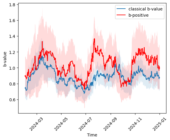
2. Plot the b-value series with a certain n_m#
>>> from seismostats.plots import plot_b_series_constant_nm
>>> mc = 1
>>> delta_m = 0.1
>>> n_m = 100
>>> ax = plot_b_series_constant_nm(mags, delta_m, mc, times, n_m=n_m, x_variable=times, color='red', plot_technique='right', label='b-positive', ax=ax, method=BPositiveBValueEstimator)
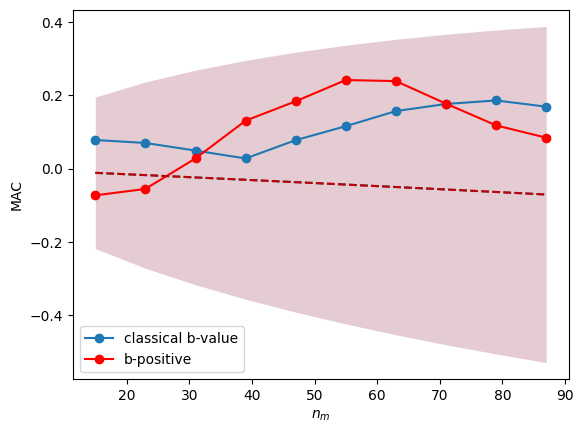
3. Visualize the autocorrelation of b-values using different n_m#
In case that it is aleady clear that the b0-value is varying, but you need to find out the length (or time) scale at which the variation is strongest, you can simply apply the b-positive method with different values of n_m. If you want to do this visually, we also have implemented a function for this.
>>> from seismostats.plots import plot_b_significant_1D
>>> mc = 1
>>> delta_m = 0.1
>>> n_m = 100
>>> ax = plot_b_series_constant_nm(mags, delta_m, mc, times, n_m=n_m, x_variable=times, color='#1f77b4', plot_technique='right', label='classical b-value')
>>> ax = plot_b_series_constant_nm(mags, delta_m, mc, times, n_m=n_m, x_variable=times, color='red', plot_technique='right', label='b-positive', ax=ax, method=BPositiveBValueEstimator)
Note that this plot follows the convention that \(n_m\) is the total number of earthquakes above the completeness that is used as input for the b-value estimation. This is done so that different b-value estimation methods can be easily compared. However, it is important to understand that for the b-positive method, the effective number of used magnitudes is around half the number of original events. This is also the reason for the larger error-band in Figure 1.
References#
Mirwald, Aron, Leila Mizrahi, and Stefan Wiemer. “How to b‐significant when analyzing b‐value variations.” Seismological Research Letters 95.6 (2024)