Notebook: Basic use of SeismoStats#
This notebook is a manual for the SeismoStats package. It is intended to be used as a reference for the basic functionality. All examples are given using the Swiss national catalog for the year 2024.
In this notebook we will show how to:
Make a catalog object
Visualisations
<ol>
    <li>Spatial plot of the seismicity</li>
    <li>Temporal plot of the seismicity</li>
    <li>Frequency-magnitude distribution plots</li>
</ol>
<li>Statistical analysis of the catalog</li>
<ol>
    <li>Estimation of the magnitude of completeness</li>
    <li>Estimation of the b-value</li>
</ol>
<li> Advanced statistical analysis</li>
<ol>
    <li>Stability of b-value over magnitudes of completeness</li>
    <li>Statistical significance of b-value variations</li>
</ol>
<li>Generate synthetic catalogs</li>
0 Import general packages#
[1]:
import pandas as pd
import matplotlib.pyplot as plt
import matplotlib.dates as mdates
import numpy as np
1 Creating a catalog object#
The columns typically contain information such as origin time, magnitude, and event location. At a minimum, a Catalog object must include a magnitude column. Common additional data columns include, but are not limited to:
time (pandas timestamp)
latitude (float)
longitude (float)
depth (float)
event_type (string)
mag_type (string)
1.1 Download a catalog from a web service#
[3]:
from seismostats import FDSNWSEventClient
from seismostats import Catalog
Start date and end date have to be defined as a datetime. In case something does not work out, the link to retrieve it manually is given back.
[4]:
# Set the time range for the catalog (year 2024)
start_time = pd.to_datetime('2024/01/01')
end_time = pd.to_datetime('2025/01/01')

# Set the geographical bounds for the catalog (Switzerland)
min_longitude = 5
max_longitude = 11
min_latitude = 45
max_latitude = 48

# Set the minimum magnitude for the events to be included in the catalog
min_magnitude = 0.5

# Query the FDSN web service
url = 'http://eida.ethz.ch/fdsnws/event/1/query'
client = FDSNWSEventClient(url)
cat = client.get_events(
    start_time=start_time,
    end_time=end_time,
    min_magnitude=min_magnitude,
    min_longitude=min_longitude,
    max_longitude=max_longitude,
    min_latitude=min_latitude,
    max_latitude=max_latitude)
The output is a catalog object
[5]:
# Show the last few rows of the catalog object
cat.tail()
[5]:
| event_type | time | latitude | longitude | depth | evaluationmode | magnitude | magnitude_type | magnitude_MLhc | |
|---|---|---|---|---|---|---|---|---|---|
| 2458 | earthquake | 2024-01-02 03:54:53.285746 | 45.869203 | 6.985509 | 6000.976562 | manual | 0.916012 | MLhc | 0.9160119489 |
| 2459 | earthquake | 2024-01-01 03:50:58.819682 | 46.854600 | 10.084163 | 229.492188 | manual | 1.411941 | MLhc | 1.411940589 |
| 2460 | earthquake | 2024-01-01 03:30:28.449568 | 45.878719 | 7.022020 | 6474.609375 | manual | 0.593754 | MLhc | 0.5937540993 |
| 2461 | earthquake | 2024-01-01 03:30:28.469196 | 45.878310 | 7.022026 | 6220.703125 | manual | 0.674713 | MLhc | 0.674713413 |
| 2462 | earthquake | 2024-01-01 02:39:21.385390 | 45.865622 | 6.997327 | 7802.734375 | manual | 0.606296 | MLhc | 0.6062956275 |
2 Seismicity Plots#
Seismicity in space
Seismicity in time
The distribution of magnitudes
2.1 Spatial visualization of seismicity#
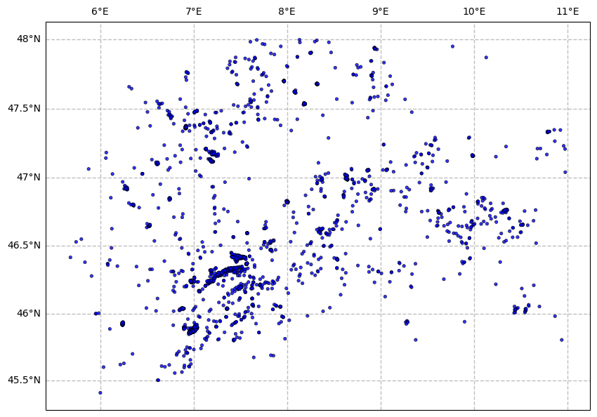
2.1.1 Basic spatial plot#
By default, the earthquakes in the catalog are a uniform size, and the same color, no map is displayed in the background, no legend is displayed.
[6]:
fig = plt.figure(figsize=(10, 10), linewidth=1)
ax = cat.plot_in_space(
    dot_smallest=0.1,
    dot_largest=10,
    dot_interpolation_power=0,
    dot_labels=False)

plt.show()
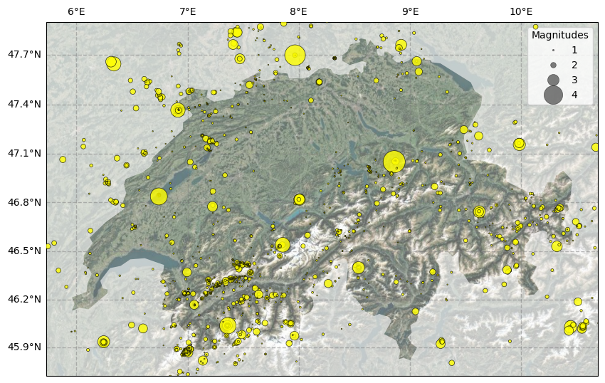
2.1.2 Adding a background map and scaling events by magnitude#
Dots size is limited to a specific range with a scaling factor specified by dot_interpolation_power. A legend is added for specified dot sizes (dot_labels).
[7]:
fig = plt.figure(figsize=(10, 10), linewidth=1)
ax = cat.plot_in_space(
    resolution='10m',
    include_map=True, # adds a map in the background
    country='Switzerland', # zooms in on Switzerland and greys out the rest of the map
    dot_smallest=1,
    dot_largest=500,
    dot_interpolation_power=3,
    dot_labels=[1,2,3,4],
    color_dots = 'yellow') # specifies the color of the dots

plt.show()
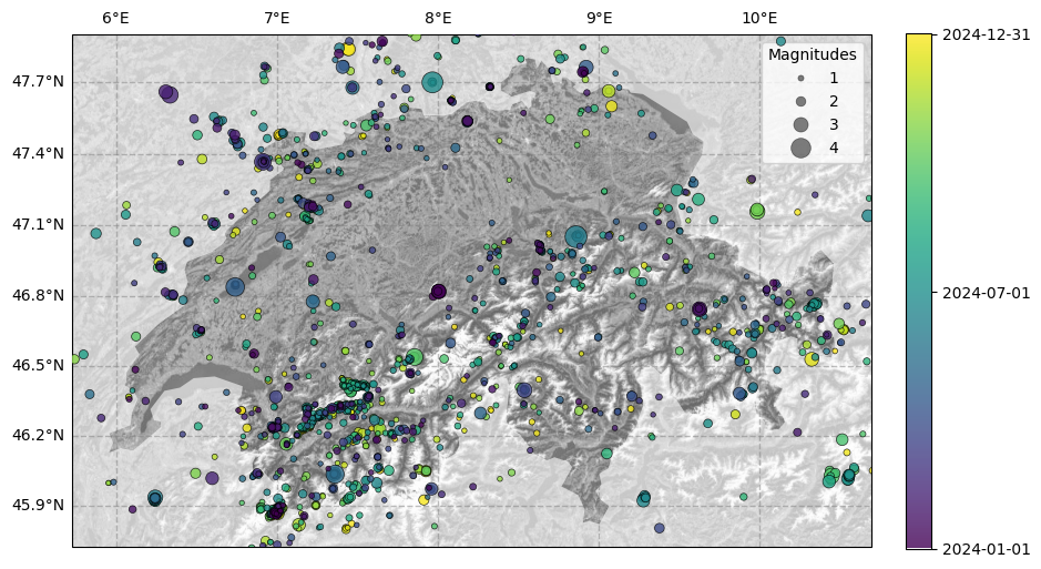
2.1.3 Temporal coloring of earthquakes#
Dots are colored by the time of the event with a color gradient specified in a colorbar (ticks can be specified with date_ticks).
[8]:
fig = plt.figure(figsize=(10, 10), linewidth=1)

ax = cat.plot_in_space(
    resolution='10m', # resolution of the map, can be '10m', '50m', '110m'
    include_map=True,
    country='Switzerland',
    color_dots=mdates.date2num(cat.time), # color the dots by time (converted to matplotlib date format)
    color_map='Greys_r', # background color for the map (default is terrain color)
    dot_labels=[1, 2, 3, 4] # legend labels for the dots
)

# Add colorbar
cbar = plt.colorbar(ax.collections[1], ax=ax, orientation='vertical', fraction=0.03, pad=0.04)

# Add dates to colorbar
date_ticks = ["2024-01-01", "2024-07-01", "2024-12-31"]
date_ticks_num = mdates.date2num(date_ticks)
cbar.set_ticks(date_ticks_num)
cbar.ax.yaxis.set_major_formatter(mdates.DateFormatter('%Y-%m-%d'))

plt.show()
2.2 Temporal visualization of seismicity#
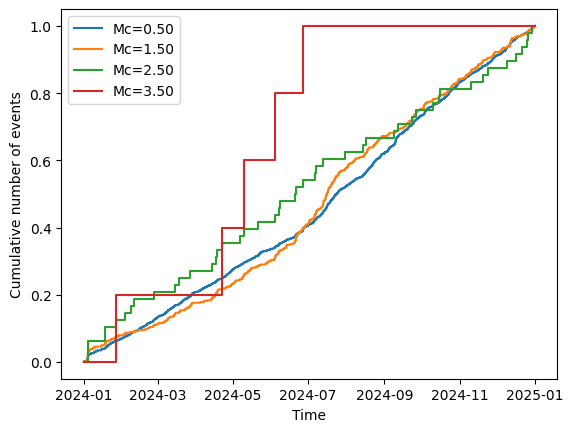
2.2.1 Cumulative count of events over time#
This plot shows the cumulative count of events over time above specific magnitude thresholds.
[9]:
# Define target magnitudes starting at 0.5 and going up to 4.0 in steps of 1.0 magnitude units
target_magnitudes = np.arange(0.5, 4.0, 1.0)

ax = cat.plot_cum_count(mcs=target_magnitudes)
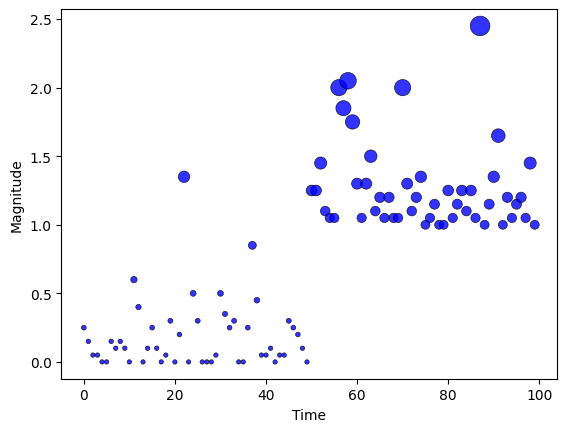
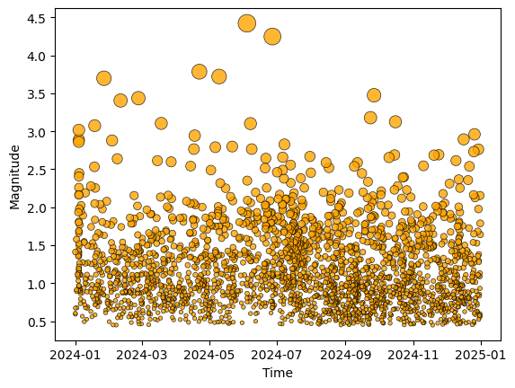
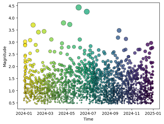
2.2.2 Timeline of magnitudes#
This plot shows the earthquakes’ magnitudes over time. By default the events all have the same color, but you can specify a color gradient based (for example) on the time of the event by specifying color_dots as a numpy array.
[10]:
# Basic version without coloring
ax = cat.plot_mags_in_time(color_dots='orange')
[11]:
# Coloring events by time
ax = cat.plot_mags_in_time(color_dots=np.arange(len(cat)))
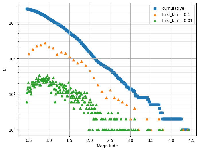
3 Frequency-Magnitude Distributions (FMD) and statistical analysis of the catalog#
FMD is a histogram-style plot that shows the number of earthquakes per magnitude bin.
3.1 Plot the FMD#
[12]:
# It is *highly* recommended to bin magnitudes to the catalogue precision before plotting
cat.bin_magnitudes(delta_m=0.01, inplace=True)

# Plot FMD
ax = plt.subplots(figsize=(8, 6))[1]

# cumulative frequency-magnitude distribution
cat.plot_cum_fmd(ax=ax)
# non-cumulative frequency-magnitude distribution with different bin sizes
cat.plot_fmd(fmd_bin=0.1, ax=ax, grid=True, label='fmd_bin = 0.1')
cat.plot_fmd(fmd_bin=0.01, ax=ax, grid=True, label='fmd_bin = 0.01')

plt.show()
Legend added to the plot.
3.2 Estimate the magnitude of completeness#
Currently, SeismoStats supports three methods to estimate the magnitude of completeness:
Maximum Curvature (MAXC)
Mc by b-value stability (MBS)
K-S distance (KS)
[13]:
# Maximum Curvature (MAXC)

# For this method a magnitude discretisation has to be selected by the user with `fmd_bin`.
# This binning might be different from the binning of the catalog; the optimal value depends on the data.
mc_maxc, _= cat.estimate_mc_maxc(fmd_bin=0.1)

# By using the a method to estimate the magnitude of completeness, the catalog is automatically updated with the estimated Mc value.
print(f'Estimated Mc using MAXC: {mc_maxc}')
print(f'Mc (currently set catalog attribute): {cat.mc}')
Estimated Mc using MAXC: 1.1
Mc (currently set catalog attribute): 1.1
[14]:
# Mc by b-value stability (MBS)
mc_stab, _ = cat.estimate_mc_b_stability(stop_when_passed=True)

print(f'Estimated Mc using MBS: {mc_stab}')
# The catalog is automatically updated with the newly estimated Mc value:
print(f'Mc (currently set catalog attribute): {cat.mc}')
return_vals: {'best_b_value': np.float64(1.063578213786541), 'mcs_tested': [0.45, 0.46, 0.47, 0.48, 0.49, 0.5, 0.51, 0.52, 0.53, 0.54, 0.55, 0.56, 0.57, 0.58, 0.59, 0.6, 0.61, 0.62, 0.63, 0.64, 0.65, 0.66, 0.67, 0.68, 0.69, 0.7, 0.71, 0.72, 0.73, 0.74, 0.75, 0.76, 0.77, 0.78, 0.79, 0.8, 0.81, 0.82, 0.83, 0.84, 0.85, 0.86, 0.87, 0.88, 0.89, 0.9, 0.91, 0.92, 0.93, 0.94, 0.95, 0.96, 0.97, 0.98, 0.99, 1.0, 1.01, 1.02, 1.03, 1.04, 1.05, 1.06, 1.07, 1.08, 1.09, 1.1, 1.11, 1.12, 1.13, 1.14, 1.15, 1.16, 1.17, 1.18, 1.19, 1.2, 1.21, 1.22, 1.23, 1.24, 1.25, 1.26, 1.27, 1.28, 1.29, 1.3, 1.31, 1.32, 1.33, 1.34, 1.35, 1.36, 1.37, 1.38, 1.39, 1.4, 1.41, 1.42, 1.43, 1.44, 1.45, 1.46, 1.47, 1.48, 1.49, 1.5, 1.51, 1.52, 1.53, 1.54], 'b_values_tested': [np.float64(0.6147350939454929), np.float64(0.6220316726527602), np.float64(0.6282246925291461), np.float64(0.6337705130377883), np.float64(0.6388937613953332), np.float64(0.642754952015558), np.float64(0.6491173818735427), np.float64(0.6556232891448491), np.float64(0.6614290921742523), np.float64(0.6670620721965064), np.float64(0.673966673128211), np.float64(0.6804414428156704), np.float64(0.6882612001669969), np.float64(0.6935310482371284), np.float64(0.6979456139885359), np.float64(0.7039734734917633), np.float64(0.708827399487406), np.float64(0.7143844171105531), np.float64(0.7190284909484651), np.float64(0.7253947441049492), np.float64(0.7322239017994069), np.float64(0.7381463198877384), np.float64(0.74309415605474), np.float64(0.7491635258069718), np.float64(0.7553264693290955), np.float64(0.7582170042725088), np.float64(0.7644532231312636), np.float64(0.7703967246619704), np.float64(0.7748375006811444), np.float64(0.7792690872173988), np.float64(0.7824606985851822), np.float64(0.7872348707470856), np.float64(0.7873435934681632), np.float64(0.7941043439277928), np.float64(0.8009734076123332), np.float64(0.807953125634993), np.float64(0.8118482358855316), np.float64(0.8152107836198433), np.float64(0.8184726505284389), np.float64(0.8216251874203099), np.float64(0.8256445235158065), np.float64(0.8275841808288222), np.float64(0.8329114170793339), np.float64(0.836673404798492), np.float64(0.8392755949271622), np.float64(0.8422528149268059), np.float64(0.8434231054847456), np.float64(0.8482834642151797), np.float64(0.8513785015060449), np.float64(0.8543240335909325), np.float64(0.8541171076912211), np.float64(0.8578279033787702), np.float64(0.8545753374414402), np.float64(0.8552262382254887), np.float64(0.8549279124095174), np.float64(0.8608715216632298), np.float64(0.8587496442128495), np.float64(0.8637073815903709), np.float64(0.8651142156369004), np.float64(0.8691133744830867), np.float64(0.8722718842586076), np.float64(0.8819624575244547), np.float64(0.8865685692957249), np.float64(0.8887583255548318), np.float64(0.8907028875105705), np.float64(0.8907686893965856), np.float64(0.8929260872442157), np.float64(0.8872557098094759), np.float64(0.8937308167652188), np.float64(0.8949651850492489), np.float64(0.9012586365519346), np.float64(0.9148714083510266), np.float64(0.9252162088036596), np.float64(0.9243569865510226), np.float64(0.9317828866520297), np.float64(0.9342781699138448), np.float64(0.9375111324727571), np.float64(0.9467508918674641), np.float64(0.9550866612711287), np.float64(0.9646008417434278), np.float64(0.9698305006171563), np.float64(0.9737851552951287), np.float64(0.9728566392131638), np.float64(0.979684103662491), np.float64(0.9889074782460171), np.float64(0.9882922716859603), np.float64(0.9883775176127556), np.float64(0.9996660079822549), np.float64(0.9978765810029513), np.float64(1.0063305366613202), np.float64(1.0078491951517161), np.float64(1.0132042722950068), np.float64(1.0139856505111975), np.float64(1.0112551629909752), np.float64(1.0123590282055928), np.float64(1.02553089726247), np.float64(1.0326458156384997), np.float64(1.0298027375306988), np.float64(1.0312073591962805), np.float64(1.035566103769404), np.float64(1.0449431872429884), np.float64(1.0543948829993623), np.float64(1.0583454069113096), np.float64(1.0638463160133087), np.float64(1.0496065155788243), np.float64(1.0496339021334304), np.float64(1.046981742839241), np.float64(1.0602670998085966), np.float64(1.0696090048453457), np.float64(1.063578213786541)], 'diff_bs': [np.float64(15.131635885844622), np.float64(14.500162768453535), np.float64(14.05271877147644), np.float64(13.69483463379221), np.float64(13.39736252631306), np.float64(13.27586792012016), np.float64(12.808596830364953), np.float64(12.319605070943204), np.float64(11.935395365665673), np.float64(11.575533542101057), np.float64(11.063108265568987), np.float64(10.61321564280138), np.float64(10.025770809948497), np.float64(11.314739938796619), np.float64(9.560421709840822), np.float64(10.720868128241959), np.float64(8.961915957335545), np.float64(10.119855386967972), np.float64(8.426335393176519), np.float64(9.465416558858529), np.float64(7.603669931953919), np.float64(8.677159153083371), np.float64(7.048982570456693), np.float64(8.111715817897084), np.float64(6.4197470260690235), np.float64(6.393597799372076), np.float64(6.08167549832864), np.float64(5.799106386140795), np.float64(5.650427450253609), np.float64(5.510708059661255), np.float64(5.477635715805673), np.float64(5.3247070537243975), np.float64(5.530482393334726), np.float64(5.226109206794217), np.float64(4.923730523835491), np.float64(4.626332088486471), np.float64(4.543903494564838), np.float64(4.494845360320316), np.float64(5.637407583859064), np.float64(4.431284575462005), np.float64(5.503778463766005), np.float64(4.400764214855867), np.float64(5.366308487336904), np.float64(4.168852037673636), np.float64(5.267875333921046), np.float64(4.141950407389241), np.float64(5.335022352545881), np.float64(4.112508346325888), np.float64(5.152098929146913), np.float64(4.069234230847452), np.float64(4.236718898856907), np.float64(4.182721714163561), np.float64(4.53866086666061), np.float64(4.671977690398312), np.float64(4.8635620639467465), np.float64(4.6767256721224575), np.float64(4.948690187727363), np.float64(4.812302382523001), np.float64(4.8856139560257175), np.float64(4.8198012561540216), np.float64(4.791605610851808), np.float64(4.412320603160712), np.float64(4.30723273784246), np.float64(4.3350361966920765), np.float64(4.377303590577061), np.float64(4.5188825154878565), np.float64(4.55036215696794), np.float64(4.981121062904464), np.float64(4.810422862436053), np.float64(4.910104125421825), np.float64(4.762086366859711), np.float64(4.274217840867053), np.float64(3.943027743134539), np.float64(4.111071339283945), np.float64(3.9134528370009893), np.float64(3.927629655750884), np.float64(3.9152323343359856), np.float64(3.6541533730858533), np.float64(3.428487270139422), np.float64(3.161407730577303), np.float64(3.0666590727035903), np.float64(3.019331334850384), np.float64(3.1438836248243835), np.float64(2.9791517232927864), np.float64(2.74022866888854), np.float64(2.835670407717723), np.float64(2.8982042120509535), np.float64(2.5707284510585335), np.float64(2.683625152378596), np.float64(2.4590201300619543), np.float64(2.45259759797295), np.float64(2.3196912665298757), np.float64(2.3353876590699167), np.float64(2.457155245476228), np.float64(2.4461612591390165), np.float64(2.0752247456132125), np.float64(1.8756817642608836), np.float64(1.9695378990168284), np.float64(1.9358516527499463), np.float64(1.8232320103338493), np.float64(1.5604857574327116), np.float64(1.3005743557182727), np.float64(1.1788360987178494), np.float64(1.0244551122424683), np.float64(1.3514525628062275), np.float64(1.332133286930673), np.float64(1.3761061219513315), np.float64(1.0545759377354078), np.float64(1.246790146946642), np.float64(0.9224874206409645)]}
Estimated Mc using MBS: 1.54
Mc (currently set catalog attribute): 1.54
UserWarning: No magnitudes in the lowest magnitude bin are present.Check if mc is chosen correctly. (base.py:119)
[15]:
# K-S distance (KS)
# This method takes longer, especially when the catalog is large.
# If Mc is known to be larger than a certain value, giving the Mc values that should be tested as an input can make the Mc estimation faster.

mc_kstest, dict = cat.estimate_mc_ks(
   mcs_test=np.arange(1.0, 3.0, 0.1), # range of Mc values to test with steps of 0.1
    p_value_pass=0.1, # p-value threshold to pass the K-S test
)

print(f"First Mc to pass the KS test: {mc_kstest:.2f}")
print(f"Associated beta value: {dict['best_b_value']:.2f}")

# The catalog is automatically updated with the newly estimated Mc value:
print(f'Mc (currently set catalog attribute): {cat.mc:.2f}')
UserWarning: Mcs to test are not binned correctly. Test might fail because of this. (estimate_mc.py:249)
First Mc to pass the KS test: 1.60
Associated beta value: 1.10
Mc (currently set catalog attribute): 1.60
[16]:
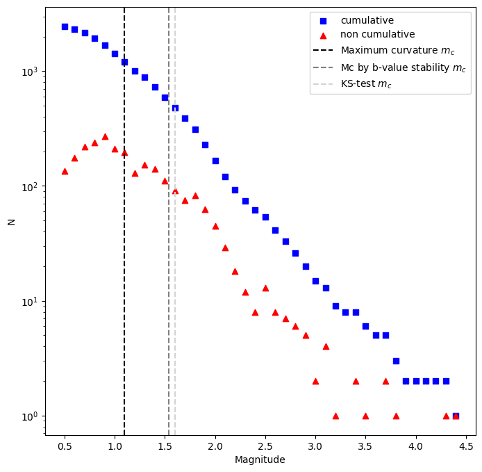
# Plot the FMD with the estimated Mc value
ax = plt.subplots(figsize=(8, 8))[1]

cat.plot_cum_fmd(fmd_bin=0.1, ax=ax, color='blue')
cat.plot_fmd(fmd_bin=0.1, ax=ax, color='red')

plt.axvline(mc_maxc, color='black', linestyle='--', label='Maximum curvature $m_c$')
plt.axvline(mc_stab, color='grey', linestyle='--', label='Mc by b-value stability $m_c$')
plt.axvline(mc_kstest, color='lightgrey', linestyle='--', label='KS-test $m_c$')

plt.legend()
plt.show()
Legend added to the plot.
3.3 Estimate the b-value#
SeismoStats supports different methods to estimate the b-value:
Classical b-value
K-S distance (KS)
Mc by b-value stability (MBS)
Note that the Mc set last will be used for the b-value estimation (in this case KS-test).
3.3.1 Classical b-value estimation#
[17]:
b_estimator = cat.estimate_b()

# The calculated b-value is stored in cat.b_value, but the estimator object contains more information:
print('Classical b-value', round(b_estimator.b_value,3))
print('Standard deviation', round(b_estimator.std,2))
print('Number of events used', b_estimator.n)
Classical b-value 1.096
Standard deviation 0.05
Number of events used 434
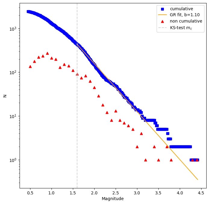
[18]:
# FMD plot with b-value
# Once a b-value is estimated and stored in cat.b_value, the FMD can be plotted with a fit:
ax = plt.subplots(figsize=(8, 8))[1]
cat.plot_cum_fmd(color='blue',ax=ax, color_line = 'orange')
cat.plot_fmd(fmd_bin=0.1, ax=ax, color='red')

plt.axvline(mc_kstest, color='lightgrey', linestyle='--', label='KS-test $m_c$')
plt.legend()
plt.show()
Legend added to the plot.
3.3.2 b-positive#
[19]:
from seismostats.analysis import BPositiveBValueEstimator
b_estimator = cat.estimate_b(method =BPositiveBValueEstimator)
print("b-positive:",round(cat.b_value,2))
b-positive: 1.13
4 Advanced statistical analysis of the catalogue#
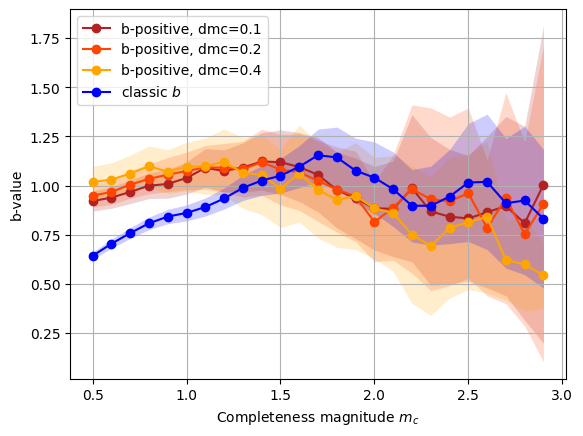
4.1 b-value stability#
[20]:
# b-value for different mangitudes of completeness
from seismostats.analysis import ClassicBValueEstimator, BPositiveBValueEstimator

mcs = np.arange(0.5, 3, 0.1)
ax = cat.plot_mc_vs_b(mcs, b_method=BPositiveBValueEstimator, dmc=0.1, color='firebrick', label='b-positive, dmc=0.1')
cat.plot_mc_vs_b(mcs, b_method=BPositiveBValueEstimator, dmc=0.2, ax=ax,  color='orangered', label='b-positive, dmc=0.2')
cat.plot_mc_vs_b(mcs, b_method=BPositiveBValueEstimator, dmc=0.4, ax=ax,  color='orange', label='b-positive, dmc=0.4')

cat.plot_mc_vs_b(mcs, b_method=ClassicBValueEstimator, ax =ax, color='blue', label='classic $b$')
[20]:
<Axes: xlabel='Completeness magnitude $m_c$', ylabel='b-value'>
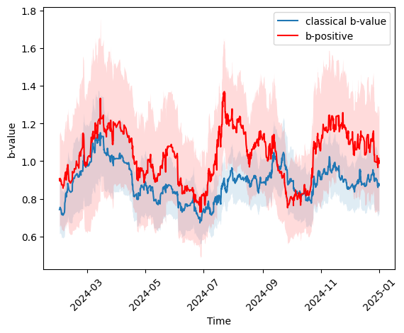
4.2 Timeseries of b-values#
Plotting the evolution of b-values (classic and positive) over time can help identify changes in seismicity patterns. One can also investigate if the variation of the b-value is larger than what one would expect just from random fluctuation of the estimate and reject a null-hypothesis of b-value being constant over time using the mean autocorrelation (see Mirwald et al., 2024).
[21]:
from seismostats.analysis import b_significant_1D
from seismostats.plots import plot_b_series_constant_nm, plot_b_significant_1D

# Parameter setting for the b-value series
mc = 1 # chosen magnitude of completeness
delta_m = cat.delta_m # binning of the magnitudes
times = cat.time
mags = cat.magnitude
n_m = 100 # number of magnitudes taken per estimate in the running window (above completeness)

ax = plot_b_series_constant_nm(mags, delta_m, mc, times, n_m=n_m, x_variable=times, color='#1f77b4', plot_technique='right', label='classical b-value')

ax = plot_b_series_constant_nm(mags, delta_m, mc, times, n_m=n_m, x_variable=times, color='red', plot_technique='right', label='b-positive', ax=ax, method=BPositiveBValueEstimator)

_ = plt.xticks(rotation=45)
ax.set_xlabel('Time')
[21]:
Text(0.5, 0, 'Time')
[22]:
# Is the b-value calculated with 100 events above completeness constant over time?
p_threshold = 0.05
p, mac, mu_mac, std_mac = b_significant_1D(mags, mc, delta_m, times, n_m, x_variable=times, method= BPositiveBValueEstimator)
print('The p-value of a constant b-value hypothesis is {:.2f}'.format(p))

print('This is significantly larger than our threshold of {:.2f}. Therefore, we cannot reject the null-hypothesis'.format(p_threshold))
The p-value of a constant b-value hypothesis is 0.42
This is significantly larger than our threshold of 0.05. Therefore, we cannot reject the null-hypothesis
UserWarning: The number of non overlapping b-value estimates is less than15. The normality assumption of the autocorrelation might not be valid. (b_significant.py:401)
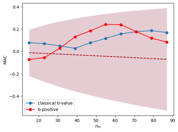
[23]:
# sort magnitudes along dimension of interest (in this case, time)
srt = np.argsort(times)
mags = mags[srt]
times = times[srt]

ax = plot_b_significant_1D(
    mags, mc, delta_m, times, x_variable=times, color = '#1f77b4', label='classical b-value')

plot_b_significant_1D(
    mags, mc, delta_m,  times, x_variable=times, method=BPositiveBValueEstimator, color = 'red', ax = ax, label='b-positive')
UserWarning: No magnitudes in the lowest magnitude bin are present.Check if mc is chosen correctly. (base.py:119)
[23]:
<Axes: xlabel='$n_m$', ylabel='MAC'>
5 Support functions#
5.1 Synthetic catalog generation#
[24]:
from seismostats.utils import simulate_magnitudes_binned

# Parameter setting for the synthetic catalog
n = 500 # number of events to simulate
b_value = 1.5 # b-value of the synthetic catalog
delta_m = 0.05 # magnitude binning of the synthetic catalog
mc = 3 # completeness of the synthetic catalog
dmc = 0.3

# Generate synthetic magnitudes
mags = simulate_magnitudes_binned(n, b_value, mc, delta_m)
cat = pd.DataFrame({'magnitude': mags})
cat = Catalog(cat)
cat.delta_m = delta_m
cat.mc = mc

# Analyse the synthetic catalog
cat.estimate_b()
print('Estimated b-value of the synthetic catalog:', round(cat.b_value,2))
Estimated b-value of the synthetic catalog: 1.52
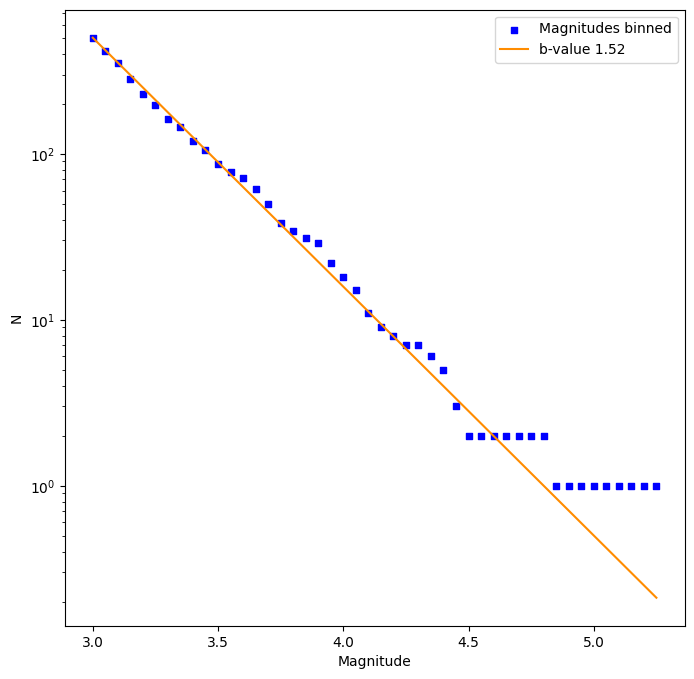
[25]:
# Plot the synthetic catalog
ax = plt.subplots(figsize=(8, 8))[1]

cat.plot_cum_fmd(ax=ax, b_value=b_value,
             color='blue', color_line = 'darkorange', label='Magnitudes binned', label_line = f'b-value {cat.b_value:.2f}', size=20)

plt.show()
Legend added to the plot.
It is also possible to generate magnitudes with varying completeness level
[26]:
from seismostats.utils import simulate_magnitudes_binned
from seismostats.plots import plot_mags_in_time
n = 100         # number of events to simulate
b_value = 1.5   # b-value of the synthetic catalog
delta_m = 0.05  # magnitude binning of the synthetic catalog
mc = np.zeros(n)          # completeness of the synthetic catalog
mc[n//2:] = 1
mags = simulate_magnitudes_binned(n, b_value, mc, delta_m)
ax = plot_mags_in_time(np.arange(len(mags)), mags)