# SeismoStats: How To
In this notebook we will show how to:#
Make a catalog object
by downloading it
by converting a csv file
<li>Plot the seismicity</li>
<li>Analyze the FMD</li>
<ol>
     <li>Plot the FMD</li>
    <li>Estimate the magnitude of completeness</li>
    <li>Estimate b-values</li>
</ol>
<li>Generate synthetic magnitudes</li>
<li>Bin magnitudes</li>
0. Import general packages#
[1]:
#%matplotlib widget
import datetime as dt
import numpy as np
import matplotlib.pyplot as plt
import pandas as pd
1. Make a catalog object#
column header |
type |
importance |
|---|---|---|
latitude |
float |
required |
longitude |
float |
required |
depth |
float |
required |
mag_type |
string |
optional |
magnitude |
float |
required |
time |
pandas timestamp |
required |
event_type |
string |
optional |
1.1 Download catalog#
[2]:
from seismostats.io.client import FDSNWSEventClient
Start date and end date have to be defined as a datetime. In case something does not work out, the link to retrieve it manually is given back.
[ ]:
start_time = pd.to_datetime('2020/01/01')
end_time = pd.to_datetime('2022/01/01')

min_longitude = 5
max_longitude = 11
min_latitude = 45
max_latitude = 48

min_magnitude = 0.5
url = 'http://eida.ethz.ch/fdsnws/event/1/query'
client = FDSNWSEventClient(url)
df = client.get_events(
    start_time=start_time,
    end_time=end_time,
    min_magnitude=min_magnitude,
    min_longitude=min_longitude,
    max_longitude=max_longitude,
    min_latitude=min_latitude,
    max_latitude=max_latitude)
The output is a catalog object
[4]:
df.tail()
[4]:
| event_type | time | latitude | longitude | depth | evaluationmode | magnitude | magnitude_type | magnitude_MLhc | magnitude_MLh | |
|---|---|---|---|---|---|---|---|---|---|---|
| 2787 | quarry blast | 2020-01-03 14:43:49.025320 | 47.187560 | 7.185673 | -683.593750 | manual | 1.213024 | MLh | NaN | 1.213023609 |
| 2788 | earthquake | 2020-01-03 14:28:09.701876 | 46.444436 | 9.104820 | 2033.203125 | manual | 0.596428 | MLh | NaN | 0.5964283368 |
| 2789 | quarry blast | 2020-01-02 08:47:20.725352 | 47.673434 | 7.585486 | 12113.281250 | manual | 0.657227 | MLh | NaN | 0.6572274734 |
| 2790 | earthquake | 2020-01-01 17:42:48.508164 | 46.031975 | 6.892110 | 5295.898438 | manual | 0.826313 | MLh | NaN | 0.8263128507 |
| 2791 | earthquake | 2020-01-01 13:43:47.626410 | 45.704174 | 7.068708 | 3302.734375 | manual | 0.824352 | MLh | NaN | 0.8243519995 |
1.2 Convert a dataframe into a catalog#
[ ]:
2. Seismicity Plots#
Seismicity in space
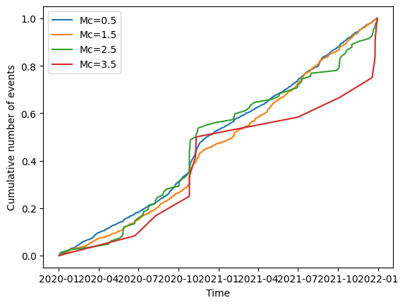
Cumulative count
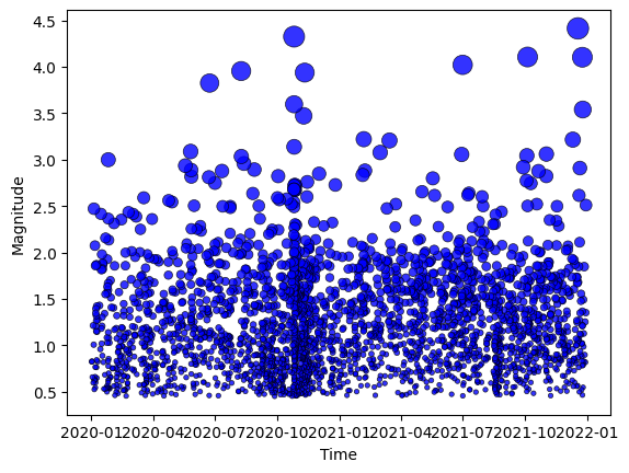
Magnitudes in time
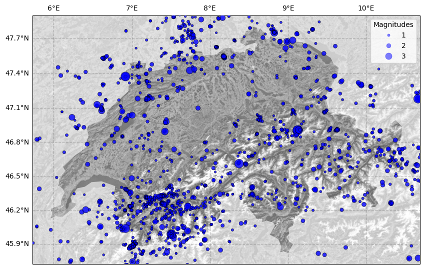
2.1. Plot in space#
[5]:
from seismostats import plot_in_space
It is possible to choose the resolutions 10, 50 and 110. Optionally you can choose the color scheme and the country of which you want to see the borders. For large areas/countries, the plotting can take some time.
[6]:
fig = plt.figure(figsize=(10, 10), linewidth=1)
ax = plot_in_space(df.longitude,
                   df.latitude,
                   df.magnitude,
                   resolution='10m',
                   include_map=True,
                   country='Switzerland',
                   colors='Greys_r',
                   dot_labels=[1,2,3])
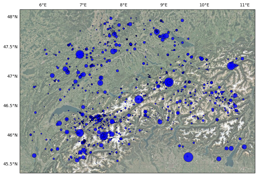
You can also choose the interpolation power and the size of the smallest and largest dot.
[7]:
fig = plt.figure(figsize=(10, 10), linewidth=1)
ax = plot_in_space(df.longitude,
                   df.latitude,
                   df.magnitude,
                   resolution='10m',
                   include_map=True,
                   dot_smallest=1,
                   dot_largest=500,
                   dot_interpolation_power=3,
                   dot_labels=None)
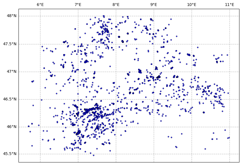
The default is that the map is not included.
[8]:
fig = plt.figure(figsize=(10, 10), linewidth=1)
ax = plot_in_space(df.longitude,
                   df.latitude,
                   df.magnitude,
                   dot_smallest=0.1,
                   dot_largest=10,
                   dot_interpolation_power=0,
                   dot_labels=False)
2.2. Plot in time#
[9]:
from seismostats import plot_cum_count, plot_mags_in_time
[10]:
ax = plot_cum_count(df.time, df.magnitude, mcs=np.arange(0.5, 4.0, 1), delta_m=0.1)
[11]:
ax = plot_mags_in_time(df.time, df.magnitude)
3. analysze the FMD#
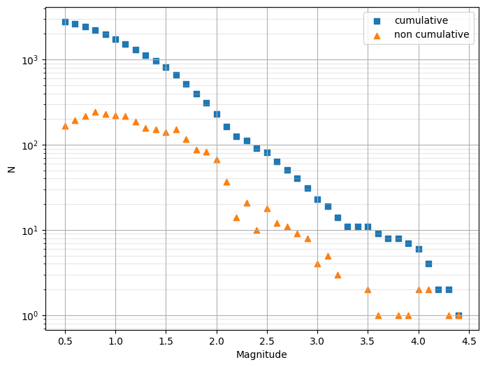
3.1 Plot magnitude distributions#
[12]:
from seismostats import plot_cum_fmd, plot_fmd
[13]:
ax = plt.subplots(figsize=(8, 6))[1]

plot_cum_fmd(df.magnitude, delta_m=0.1, ax=ax)
plot_fmd(df.magnitude, ax=ax, grid=True)

plt.show()
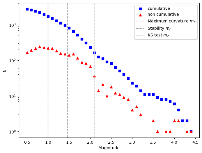
3.2 Estimate completeness magnitude#
[14]:
from seismostats.analysis.estimate_mc import mc_ks, mc_max_curvature, mc_by_bvalue_stability
from seismostats.utils.binning import bin_to_precision
[15]:
mc_stab, best_b, mcs_test, bs, diff_bs = mc_by_bvalue_stability(df.magnitude, delta_m=0.01, stop_when_passed=True)
print(f'Stability method: Mc = {mc_stab:.2f}')
Stability method: Mc = 1.46
[16]:
mc = mc_max_curvature(df.magnitude, delta_m=0.1)
print(f'Maximum curvature method: Mc = {mc:.1f}')
Maximum curvature method: Mc = 1.0
[ ]:
mc_kstest, beta_kstest, mcs_tested, betas, ks_ds, ps = mc_ks(
    bin_to_precision(df.magnitude, 0.1),
    delta_m=0.1,
    p_value_pass=0.1,
)

print(f"KS test method:")
print("Tested Mc values:", mcs_tested)
print("First Mc to pass the KS test:", mc_kstest)
print(f"Associated beta value: {beta_kstest:.2f}")
KS test method:
Tested Mc values: [np.float64(0.5), np.float64(0.6), np.float64(0.7), np.float64(0.8), np.float64(0.9), np.float64(1.0), np.float64(1.1), np.float64(1.2), np.float64(1.3), np.float64(1.4), np.float64(1.5), np.float64(1.6), np.float64(1.7), np.float64(1.8), np.float64(1.9), np.float64(2.0), np.float64(2.1)]
First Mc to pass the KS test: 2.1
Associated beta value: 2.01
This method takes longer, especially when the magnitude sample is large.
If Mc is known to be larger than a certain value, giving the Mc values that should be tested as an input can make the Mc estimation faster.
[ ]:
# if Mc is known to be larger than or equal to 1.0

mc_kstest, beta_kstest, mcs_tested, betas, ks_ds, ps = mc_ks(
    bin_to_precision(df.magnitude, 0.1),
    mcs_test=bin_to_precision(np.arange(1.0, 3.0, 0.1), 0.1),
    delta_m=0.1,
    p_value_pass=0.1,
)

print("Tested Mc values:", mcs_tested)
print("First Mc to pass the KS test:", mc_kstest)
print(f"Associated beta value: {beta_kstest:.2f}")
Tested Mc values: [np.float64(1.0), np.float64(1.1), np.float64(1.2), np.float64(1.3), np.float64(1.4), np.float64(1.5), np.float64(1.6), np.float64(1.7), np.float64(1.8), np.float64(1.9), np.float64(2.0), np.float64(2.1)]
First Mc to pass the KS test: 2.1
Associated beta value: 2.01
[19]:
ax = plt.subplots(figsize=(8, 6))[1]

plot_cum_fmd(df.magnitude, delta_m=0.1, ax=ax, color='blue')
plot_fmd(df.magnitude, ax=ax, color='red')

plt.axvline(mc, color='black', linestyle='--', label='Maximum curvature $m_c$')
plt.axvline(mc_stab, color='grey', linestyle='--', label='Stability $m_c$')
plt.axvline(mc_kstest, color='lightgrey', linestyle='--', label='KS-test $m_c$')

plt.legend()
plt.show()
3.3 Estimate the b-value#
[20]:
from seismostats import estimate_b, bin_to_precision
from seismostats.plots.statistical import plot_mc_vs_b
[21]:
delta_m = 0.1
mags = df.magnitude
mags = bin_to_precision(mags, delta_m)
[22]:
b_estimate, error = estimate_b(mags[mags>=mc], mc=mc, delta_m=delta_m, return_std=True, b_parameter='b_value')

b_estimate2, error = estimate_b(mags[mags>=mc_kstest], mc=mc_kstest, delta_m=delta_m, return_std=True, b_parameter='b_value')
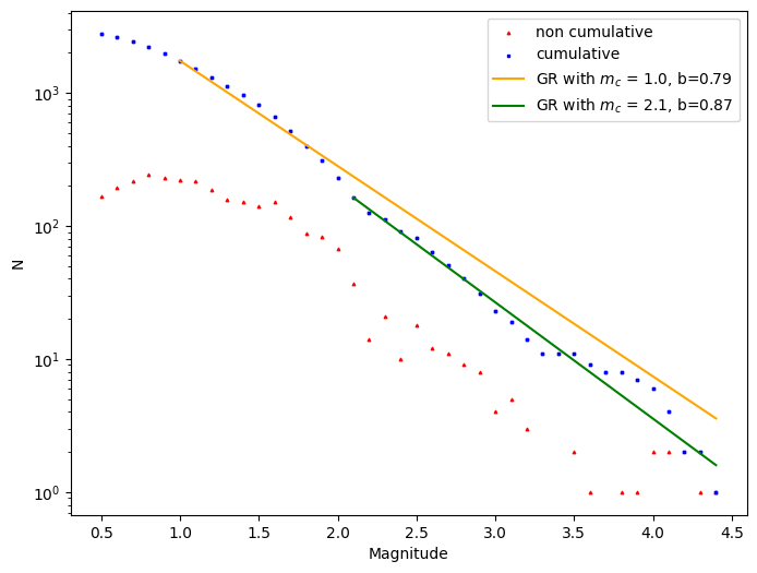
[23]:
ax = plt.subplots(figsize=(8, 6))[1]

plot_fmd(df.magnitude, ax=ax, color='red', size=3)

plot_cum_fmd(df.magnitude, delta_m=0.1, ax=ax, color=['blue', 'orange'], b_value=b_estimate, mc=mc,
             size=3, legend=['cumulative', r'GR with $m_c$ = {:.1f}'.format(mc)])
plot_cum_fmd(df['magnitude'], delta_m=0.1, ax=ax, b_value=b_estimate2, mc=mc_kstest, color = ['blue', 'green'],
             size=3, legend=['_', r'GR with $m_c$ = {:.1f}'.format(mc_kstest)])

plt.show()
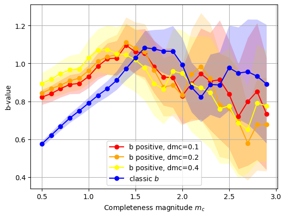
We can also plot the b-value for different mc:
[24]:
from seismostats.analysis.bvalue import ClassicBValueEstimator, BPositiveBValueEstimator

mcs = np.arange(0.5, 3, 0.1)
ax = plot_mc_vs_b(mags, mcs, delta_m, b_method=BPositiveBValueEstimator, dmc=0.1, color='red', label='b positive, dmc=0.1')
plot_mc_vs_b(mags, mcs, delta_m, b_method=BPositiveBValueEstimator, dmc=0.2, ax=ax,  color='orange', label='b positive, dmc=0.2')
plot_mc_vs_b(mags, mcs, delta_m, b_method=BPositiveBValueEstimator, dmc=0.4, ax=ax,  color='yellow', label='b positive, dmc=0.4')

plot_mc_vs_b(mags, mcs, delta_m, b_method=ClassicBValueEstimator, ax =ax, color='blue', label='classic $b$')
[24]:
<Axes: xlabel='Completeness magnitude $m_c$', ylabel='b-value'>
3.4 Check if the b-value changes significantly#
Once we picked a fitting completeness, we might also want to see how the b-value changes with time (or along any other dimension)
[4]:
from seismostats.analysis.b_significant import b_significant_1D
from seismostats import bin_to_precision
from seismostats.plots.statistical import plot_b_series_constant_nm, plot_b_significant_1D
from scipy.stats import norm

from seismostats.analysis.bvalue import BPositiveBValueEstimator
[5]:
mc = 1.0
delta_m = 0.1

times = df['time'].values
mags = df['magnitude'].values
mags = bin_to_precision(mags, delta_m)
[6]:
n_m = 100 # number of magnitudes taken per estimate in the running window

idx = mags >= mc
ax = plot_b_series_constant_nm(mags[idx], delta_m, mc, times[idx], n_m=n_m,x_variable=times[idx], color='#1f77b4', plot_technique='right', label='classical b-value')

ax = plot_b_series_constant_nm(mags[idx], delta_m, mc, times[idx], n_m=n_m,x_variable=times[idx], color='red', plot_technique='right', label='b-positive', ax=ax, b_method=BPositiveBValueEstimator)

_ = plt.xticks(rotation=45)
ax.set_xlabel('Time')
[6]:
Text(0.5, 0, 'Time')
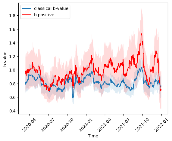
Looking at the time-series above, one could be interested if the variation of the b-value is larger than what one would expect just from random fluctuation of the estimate. In other words, we want to know if we can reject the null-hypothesis that the true b-value is constant. For this, we can apply the method of Mirwald et. al., 2024.
For this, we estimate the mean autocorrelation (MAC). The MAC can then be used to estimate a p-value. If the p-value is smaller than a threshold (which we have to choose, often 0.05 is used), then we can reject the null-hypothesis, and we are justified to believe that the b-vlue is in fact changing.
[7]:
n_m = 100

idx = mags >= mc
p, mac, mu_mac, std_mac = b_significant_1D(mags[idx], mc, delta_m, times[idx], n_m)

# b-positive
p, mac, mu_mac, std_mac = b_significant_1D(mags[idx], mc, delta_m, times[idx], n_m, method= BPositiveBValueEstimator)
/Users/aron/polybox/Projects/SeismoStats/env/lib/python3.11/site-packages/seismostats/analysis/b_significant.py:367: UserWarning: The number of subsamples is less than 25. The normality assumption of the autocorrelation might not be valid.
  warnings.warn(
[8]:
p_threshold = 0.05
print('The p-value of a constant b-value hypothesis is {:.2f}'.format(p))
print('This is significantly larger than our threshold of {:.2f}. Therefore, we cannot reject the null-hypothesis'.format(p_threshold))
The p-value of a constant b-value hypothesis is 0.13
This is significantly larger than our threshold of 0.05. Therefore, we cannot reject the null-hypothesis
We found that the temporal variation was not significant, therefore further interpretation of how the b-value changes with time might not be reasonable to do. But this was specifically using a certain number of magnitudes per estimate. Maybe there is some other scale, where the b-value does change significantly?
We can test this easily by applying the same method with different n_m.
[9]:
ax = plot_b_significant_1D(
    mags, times, mc, delta_m, x_variable = times, color = '#1f77b4', label='classical b-value', ax = ax)

plot_b_significant_1D(
    mags, times, mc, delta_m, x_variable = times, color = 'red', b_method=BPositiveBValueEstimator, ax = ax, label='b-positive')
/Users/aron/polybox/Projects/SeismoStats/env/lib/python3.11/site-packages/seismostats/analysis/bvalue/base.py:91: UserWarning: No magnitudes in the lowest magnitude bin are present.Check if mc is chosen correctly.
  warnings.warn(
classical b-value
check
b-positive
check
[9]:
<Axes: xlabel='Time', ylabel='b-value'>
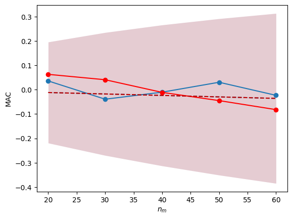
We found that in fact, the variation of the b-value is not significant for any scale.
4. Generate and bin synthetic earthquakes#
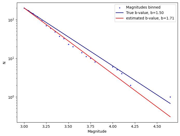
First we need to define the number of earthquakes, the b-value and the completeness magnitude. If binnning is applied, it is important to generate the magnitudes half a bin smaller than the smallest magnitude, otherwise the first bin will contain only half the events. For the b-value, note that beta is defined as the natural logarithm equivalent of the b-value.
[20]:
from seismostats import simulate_magnitudes_binned, estimate_b
from seismostats import plot_cum_fmd
import matplotlib.pyplot as plt
[16]:
n = 200
b_value = 1.5
delta_m = 0.05
mc = 3
dmc = 0.3
Now we can generate a synthetic magnitude distribution:
[17]:
mags = simulate_magnitudes_binned(n, b_value, mc, delta_m)
In order to bin the magnitudes, we just need to define the step-size:
[18]:
b_estimate, error = estimate_b(mags, mc=mc, delta_m=delta_m, return_std=True, b_parameter='b_value')
We can plot the original and binned magnitudes and their respective b-value estimates now. Note that we choose the bin position to be left in order to align the binned and the original magnitudes.
[19]:
ax = plt.subplots(figsize=(8, 6))[1]

plot_cum_fmd(mags, ax=ax, b_value=b_value, mc=mc - delta_m/2,
             color=['blue', 'darkblue'], legend=['Magnitudes binned', 'True b-value'], size=3)
plot_cum_fmd(mags, ax=ax, b_value=b_estimate, mc=mc - delta_m/2,
             color=['blue', 'red'], legend=['_', 'estimated b-value'], size=3)

plt.show()